Early warning systems for vector-borne diseases based on predictive modeling can play a critical role in public health decision making by enabling proactive interventions such as vector control and resource allocation. Multiple modelling approaches have been applied for VBD forecasting, like statistical models, machine learning approaches, and mechanistic models. However, the assessment of performance of these models is often limited to a few standard metrics, which does not capture their operational utility for a public health use case. VBD-ModelBench provides an evaluation framework to benchmark predictive models across multiple metrics, lead times, and operationally relevant scenarios, so that model selection and implementation is based on operational readiness rather than one aggregate error score.
For each model, forecasts are assessed over different evaluation periods, and spatial units. Results are then stratified to analyse performance differences that aggregate scores might not reveal, for example differences across regions, seasonal periods, case-load regimes, or forecast horizons.
The main sections describe the recursive forecast generation setup, the operationally relevant aspects of the evaluation method in addition to standard error-based evaluation.
Forecast Generation
Multiple modeling approaches can be utilized for forecasting vector-borne diseases. Some of which are detailed here. Each model can then have multiple input features: dynamic like recent reported cases of the disease, meteorological variables or static like demographic or geo-spatial datasets etc. Once the models are trained, forecasts are generated on a test set which will later be evaluated to quantify the performance of the model.
To generate forecasts, we employ a sliding window approach where at each forecast origin, we predict the next H weeks. Each model will predict for a certain forecast horizon H and will require observed data from a lagging window Lx for dynamic features, (say reported cases or meteorological data). The models can also have static features that do not evolve over time.
We first set up notations for the input features (dynamic and static) and parameters:
| Variable | Description | Remarks |
|---|---|---|
| z | Absolute time index | z ∈ {0,...,N} |
| Oz | Observed cases at time z | |
| Pz | Predicted cases at time z | |
| Wz | Dynamic Features like weather variables at time z | |
| Iz | Static Features | |
| H | Forecast horizon (number of total time steps predicted per run) | |
| h | Lead time (step within the forecast horizon) | h ∈ {0,...,H} |
| s | Sliding window shift | s ≤ H |
| Lx | Lag value for any feature x | |
| tk | Origin of the k-th forecast window | |
| K | Total number of possible sliding windows | |
| k | Index of the sliding window | k ∈ {0,...,K-1} |
For models that use Lagged Reported Cases as Feature
Models where recently reported cases are also an input feature can employ a recursive forecasting method (such that the prediction from the model is an input for the next prediction.)in addition to the sliding window approach. For example, for a weekly scale model, at each forecast origin we predict the next H weeks. For the first future week, the model can use the observed reported cases from the previous week. For later future weeks(two and beyond), reported cases from the previous week are no longer known, so the model uses its own earlier predictions as inputs. This makes the evaluation closer to operational settings, where future case data is unavailable.
Sliding Window
We use a sliding window approach where the forecast window of length H (and hence the origin t_k) shifts by time step s:
where Ytk + h − 1tk, are the lagged cases which are derived in the following way:
Lagged cases: For window k, at origin tk, to predict lead time h, the model will require L lagged case values ending at tk + h − 1. Fix a forecast horizon H with lag L, and sliding window 0 ≤ k ≤ K. For predicting the case at origin tk we use the
as the L-lagged case values. Suppose we wish to predict the cases on tk + h for some h = 1, 2, …, H− 1, we will inductively on h use the following as L lagged case values
to predict tk + h, where Oz are the reported cases and Pzk are the predicted cases for the previous h − 1 days when h ≥ 1. The following is an example representation for the above method:
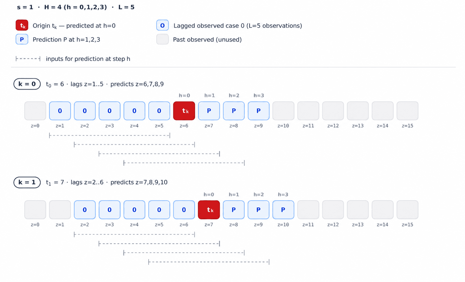
Figure
At h=0, all L=5 inputs are real observations. As h grows, each new prediction replaces an observation, compounding the error with each step. By h=3, three of the five inputs are predictions. Each new window, k, resets to all-observed inputs.
For models that do not use Lagged Reported Cases as Feature
The sliding window approach can also be employed for models that do not use lagged reported cases as features and instead only use other dynamic features like meteorological variables. Only the predictions expression changes as follows(since there are no case data inputs):
The sliding window method results in multiple predictions for the same week which helps evaluating model performance for each week at different lead times(as explained later).
Evaluation Methodology
The evaluation methodology uses multiple metrics, including both standard and operationally relevant metrics. It is based on a stratified evaluation process, where models are benchmarked across different lead times, outbreak regimes.
Operational Relevance
Standard error metrics like Root Mean Squared Error and Normalised Root Mean Squared Error focus on numeric differences between predicted and observed case counts which are insufficient to evaluate models that are to be used for public health decision making processes. They are useful as ad hoc metrics, but can hide under-prediction and regime-specific failure. While evaluating models for implementation, it is important to understand the requirements of the health system and the context in which the model will be used.
Operational metrics evaluate whether forecast will be useful for resource allocation and planning. Operational metrics assess whether the model captures actionable signals such as risk categories, direction of change, timing of increases, and under-prediction during high-burden periods.
- Reliability: If the model is being used to predict for a longer time horizon, the degradation in performance should be assessed to ensure reliability
- Capturing the trend: If the models are to be used for early warning, they should be evaluated on their ability to capture the peak and rise in cases.
- Resource Allocation: If forecasts are used to allocate resources, then the models should be able to accurately predict the total burden.
- Data availability: If recent case reports arrive late, models should be evaluated under the same reporting-delay constraints.
Stratified Evaluation
The models are evaluated across different strata like:
Lead times
To understand on how far ahead the forecast remains reliable and how much it degrades. A model that performs well one week ahead may not be useful for preparedness if its skill collapses at longer lead times, say 4 weeks ahead.
Case Percentile
To assess model performance across varying levels of disease burden (low vs. high). Case counts during the evaluation period are divided into three categories: Low, representing values at or below the 33rd percentile; Medium, representing values between the 33rd and 67th percentiles; and High, representing values above the 67th percentile.
Season
To compare model metrics across seasons: pre-monsoon, monsoon, and post-monsoon. This will show whether a model performs well during the peak transmission season or only in the off-season.
Regions
Evaluate model performance across different regions to ensure the model works well in all regions.
Risk Categorisation
Evaluate low, moderate, high, and critical risk classes separately. Since misclassifying a high-risk period as low risk is more costly.
Metric Categories
We use multiple metrics; both Standard Metrics and Operationally Relevant Metrics, since as discussed a single metric is not enough to capture all the aspects of forecast performance. Additionally, all these metrics are stratified by the regimes above
Magnitude accuracy
Root Mean Squared Error and Normalised Root Mean Squared Error estimate how far predicted case counts are from observed counts.
Bias and LinEx loss
Generally, under prediction is more costly than over-prediction in a health system. Bias identifies systematic under- or over-prediction and LinEx loss penalizes the more costly direction, here, underprediction.
Trend capture
Pearson and trajectory correlation test whether forecasts track the rise, peak, and decline of cases.
Risk-band metrics
Accuracy, precision, recall, and F1 evaluate whether forecasts classify actionable risk levels(low, medium, high, critical) correctly.
Benchmarking Models
We benchmark models against a naive persistence baseline to understand whether the models provide actionable improvement. We calculate skill scores to quantify this improvement.
All comparisons use a global common cohort. An observation is included only when it is available for every benchmark model, matched by evaluation period, forecast horizon, lead time, region, forecast origin, and target week. The selected model and the naive-persistence baseline are therefore evaluated on the same observations. The evaluation output records the sample count for every reported metric and stratum.
Naive Persistence: The prediction at week t + h equals the observed value at week t - k for a given lag k and, lead time, h :
Skill Score can be used to quantify the performance of the model relative to the naive/baseline model. A positive skill score indicates improvement over the baseline For metrics where higher is better, such as accuracy, recall, F1, trajectory correlation, and direction accuracy, skill is computed as:
For metrics where lower is better, such as LinEx, skill is computed as:
Qualification Criteria for the Ensemble of models
No single model is optimal across all regimes or geographies, hence an ensemble of models is used. The qualification criteria for a model to be included in the Ensemble must be context-driven. Model selection should consider the following aspects:
Appendix
Standard Metrics :
Let yi denote the true values, ŷi the predicted values, and n the number of samples.
Root Mean Squared Error (RMSE)
RMSE measures the square root of the average squared differences between the predicted and actual values. It penalizes larger errors more heavily due to squaring, making it sensitive to outliers. Lower RMSE indicates better model performance.
Normalized Root Mean Squared Error (NRMSE)
NRMSE normalizes RMSE by the mean of the observed values, making it scale-independent. This allows for comparisons across regions(here, zones) and models.
Coefficient of Determination (R2)
R2 measures the proportion of variance in the observed data that is explained by the model. Values closer to 1 indicate better fit.
Pearson Correlation Coefficient (rho)
Pearson correlation coefficient measures the linear relationship between the true and predicted values. It ranges from -1 (perfect negative correlation) to 1 (perfect positive correlation), with 0 indicating no linear relationship. A higher correlation indicates that the model can capture trends (rises/falls) in the data.
Operational Metrics
Let yi denote the observed case count and ŷi denote the forecast for observation i. Let bi in {1,2,3,4} denote the observed risk band and b̂i in {1,2,3,4} denote the predicted risk band, where the bands correspond to Low, Moderate, High, and Critical risk.
Risk-Band Classification Metrics
For risk-band evaluation, forecasts are first converted into discrete risk bands using predefined endemic-channel thresholds. A confusion matrix C is then constructed, where
Precision answers: when the model predicts a given risk band, how often is it correct? Recall answers: when that risk band actually occurs, how often does the model detect it? F1 balances these two quantities and is useful when missing high-risk periods and over-alerting both matter.
where N is the total number of evaluated observations.
Bias
Bias measures the average tendency of predictions to overestimate or underestimate the true values. A positive bias indicates overprediction, while a negative bias indicates underprediction.
LinEx Loss
Here, ln denotes the natural logarithm and alpha = 0.75. Applying LinEx to log-transformed case counts keeps the exponential term numerically stable while retaining asymmetric penalties.
Underprediction gives e > 0 and is penalised more heavily than overprediction, where e < 0. Loss approaches zero as e approaches zero, and alpha controls the degree of asymmetry. This definition matches the canonical Python evaluator used to produce the interactive results.
Trajectory Correlation
Defined when n >= 3, std(y_true) > 0, std(y_pred) > 0
Arrays must be sorted chronologically before computing.
References
- Zellner, A. (1986). Bayesian estimation and prediction using asymmetric loss functions (opens in a new tab). Journal of the American Statistical Association, 81(394), 446–451.
- World Health Organization. (2016). Technical handbook for dengue surveillance, outbreak prediction/detection and response (opens in a new tab). World Health Organization.